


FinOps for Data Engineering: Architecting Pipelines with Cost in Mind
TLDR/key takeaways:
- Snowflake cost optimization rarely requires a rewrite, because most warehouse waste comes from default settings, full table scans, and repeated computation that nobody revisited as data volumes grew.
- Snowflake bills warehouses per second with a 60-second minimum every time a warehouse resumes, so when queries arrive more often than once a minute, an aggressive auto-suspend timeout can cost more than leaving the warehouse running.
- On BigQuery on-demand pricing, partitioning a large table to match its query filters can cut the bytes each query scans, and therefore the bill, by more than 90%.
- The highest-leverage first step on Snowflake or BigQuery is visibility: tag queries by team and pipeline, then audit the ten most expensive queries from the last 30 days.
Why did the warehouse bill climb when nothing broke?
Cloud data warehouses don’t get expensive because they’re poorly designed. They get expensive because their defaults favor flexibility and time-to-value over cost. A pipeline that ran cheaply at 10 GB of daily data can quietly become expensive at 10 TB, not because anything failed, but because nobody revisited the original design decisions as the data grew. Finding those decisions is the real work of Snowflake cost optimization, and the same levers cut BigQuery costs.
This guide is for data engineers, platform engineers, and engineering managers who want the bill back under control without re-architecting everything. It covers why costs climb, the table design and compute changes that bring them down, and how to audit spend and start a FinOps practice without a big-bang rewrite.
Why cloud data warehouse costs climb as pipelines scale
Three patterns drive most of the compute bill on both platforms, and none of them is a platform flaw. Warehouses bill for compute consumed (execution time, warehouse size, or slots) plus storage, so anything that makes a query read or run more than necessary lands on the invoice.
- Full table scans instead of pruned scans. If a table isn’t partitioned or clustered to match how it’s queried, a query filtering for a single day can still scan the table’s entire history.
- Compute sized for peak load. Fixed-size warehouses and generous auto-suspend timeouts or baseline slots add idle cost across every daily pipeline.
- Redundant computation. Dashboards and scheduled jobs recompute the same aggregations from raw data several times a day, even when nothing changed.
Stop paying to scan and recompute data you don’t need
The principle is the same on both platforms: let the WHERE clause eliminate physical data before it’s read, and compute a repeated aggregation once instead of on every refresh.
Partitioning in BigQuery
A daily pipeline that scans a 2 TB events table costs about $375 a month at BigQuery’s on-demand rate of $6.25 per TiB (illustrative, before the monthly free tier). Partition that table by event date and a typical query scans about 80 GB instead, which brings the same workload to roughly $14 a month. That is a 96% reduction from one DDL change.
BigQuery prunes partitions whenever a query filters on the partitioning column, so a filter on created_at >= '2026-07-01' reads only July onward rather than three years of history.
-- BigQuery: partition and cluster at creation time
CREATE TABLE analytics.events
PARTITION BY DATE(created_at)
CLUSTER BY customer_id
OPTIONS (require_partition_filter = TRUE)
AS SELECT * FROM raw.events;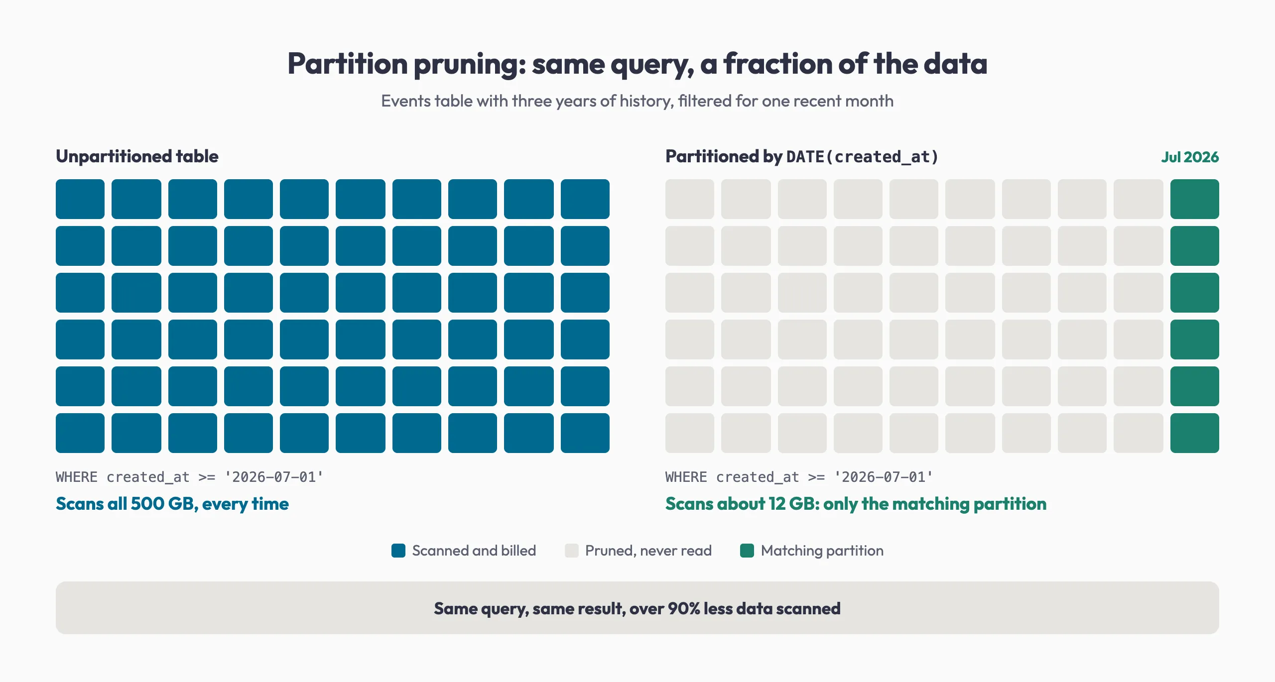
require_partition_filter makes BigQuery reject any query without a partition filter, so nobody triggers a full scan by accident. Clustering on customer_id prunes further within each partition.
Clustering keys in Snowflake
Clustering keys lay out micro-partitions so rows with similar values sit together, so a query filtering on region = 'APAC' reads far fewer of them.
-- Snowflake: add clustering to an existing table
ALTER TABLE analytics.events CLUSTER BY (region, event_date);

-- Check clustering effectiveness
SELECT SYSTEM$CLUSTERING_INFORMATION('analytics.events', '(region, event_date)');
A high average_depth in that output means the table is poorly clustered. Be selective, though. Snowflake recommends clustering keys mainly for tables in the multi-terabyte range that are filtered the same way often, because reclustering itself consumes credits.
Materialize repeated aggregations
Both platforms cache results for exact repeat queries, but only when the query text and data are identical. The bigger win is intentional materialization. A nightly dbt job that builds a daily_revenue_by_product table, ideally with one of the incremental strategies in dbt, lets dashboards read a small summary table instead of re-scanning raw transactions on every page load.
BigQuery materialized views refresh in the background and read only what changed where possible. Snowflake materialized views are maintained automatically too, which consumes credits and requires Enterprise Edition.
-- BigQuery materialized view
CREATE MATERIALIZED VIEW analytics.daily_revenue_by_product AS
SELECT
  DATE(order_timestamp) AS order_date,
  product_id,
  SUM(revenue) AS total_revenue,
  COUNT(*) AS order_count
FROM raw.orders
GROUP BY 1, 2;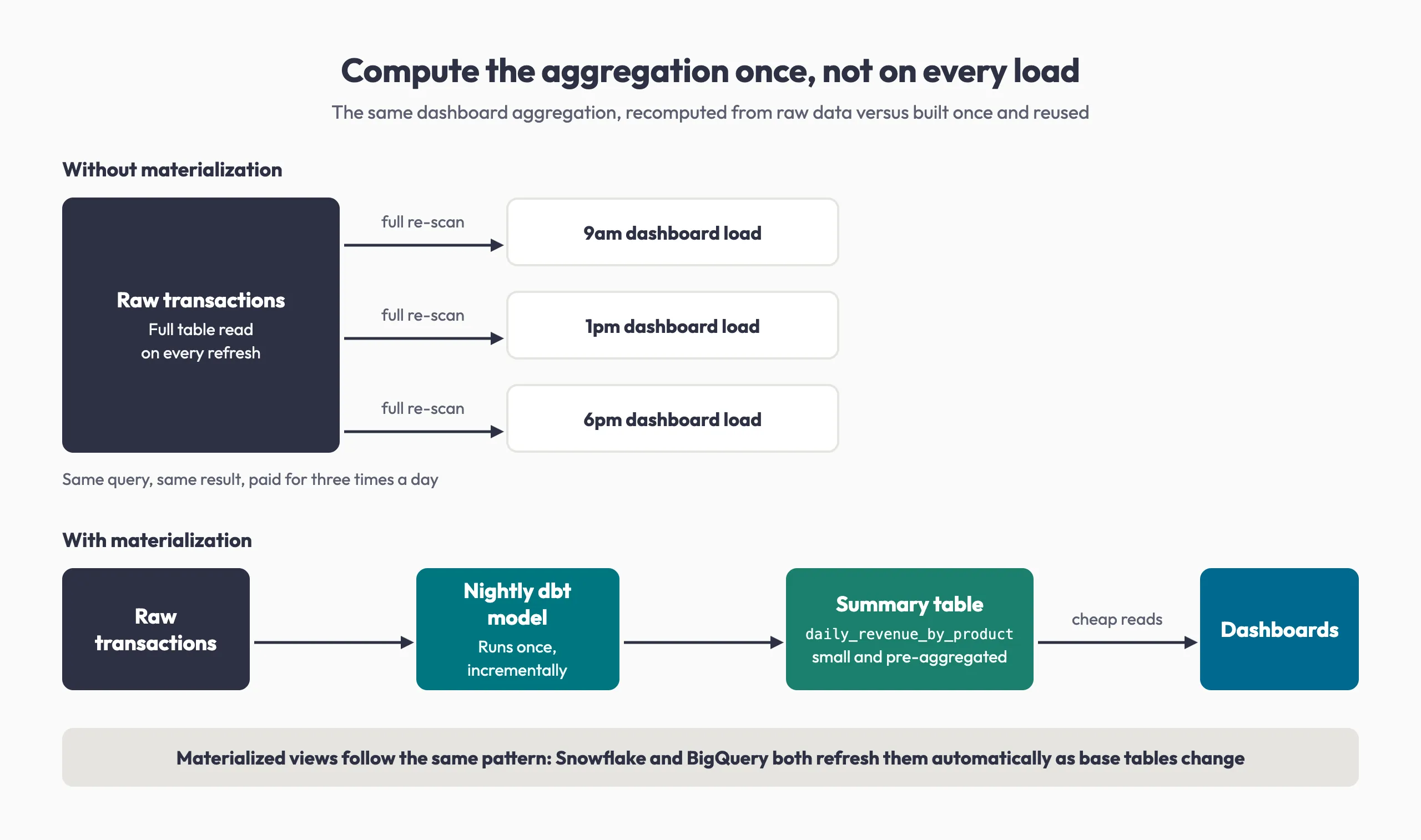
This is a design decision, not a platform feature: someone has to find the queries that repeat the same logic.
Right-size compute on Snowflake and BigQuery
On Snowflake, the auto-suspend timeout is the setting most likely to be wrong in both directions. Two mechanics explain why.
The 60-second minimum on resume. A warehouse bills per second while running, but each start or resume is charged for at least 60 seconds. Picture 5-second queries arriving every 40 seconds on a warehouse with a 30-second timeout. It suspends between queries, then resumes for the next one, and every resume is billed a full 60 seconds: 60 seconds billed for every 40 seconds of wall time. Left running, the same warehouse bills 40. When queries arrive more often than once a minute, a short timeout makes the warehouse thrash.
Suspending drops the warehouse cache. A running warehouse caches the table data its queries touch, and Snowflake drops that cache on suspend, so the first queries after a resume run slower. On BI workloads, aggressive suspension trades a small idle saving for slower dashboards.
-- Snowflake: set auto-suspend per workload type
-- ETL warehouse: suspend quickly after the batch completes
ALTER WAREHOUSE etl_wh SET AUTO_SUSPEND = 60;

-- BI warehouse: keep the cache warm for interactive users
ALTER WAREHOUSE bi_wh SET AUTO_SUSPEND = 600;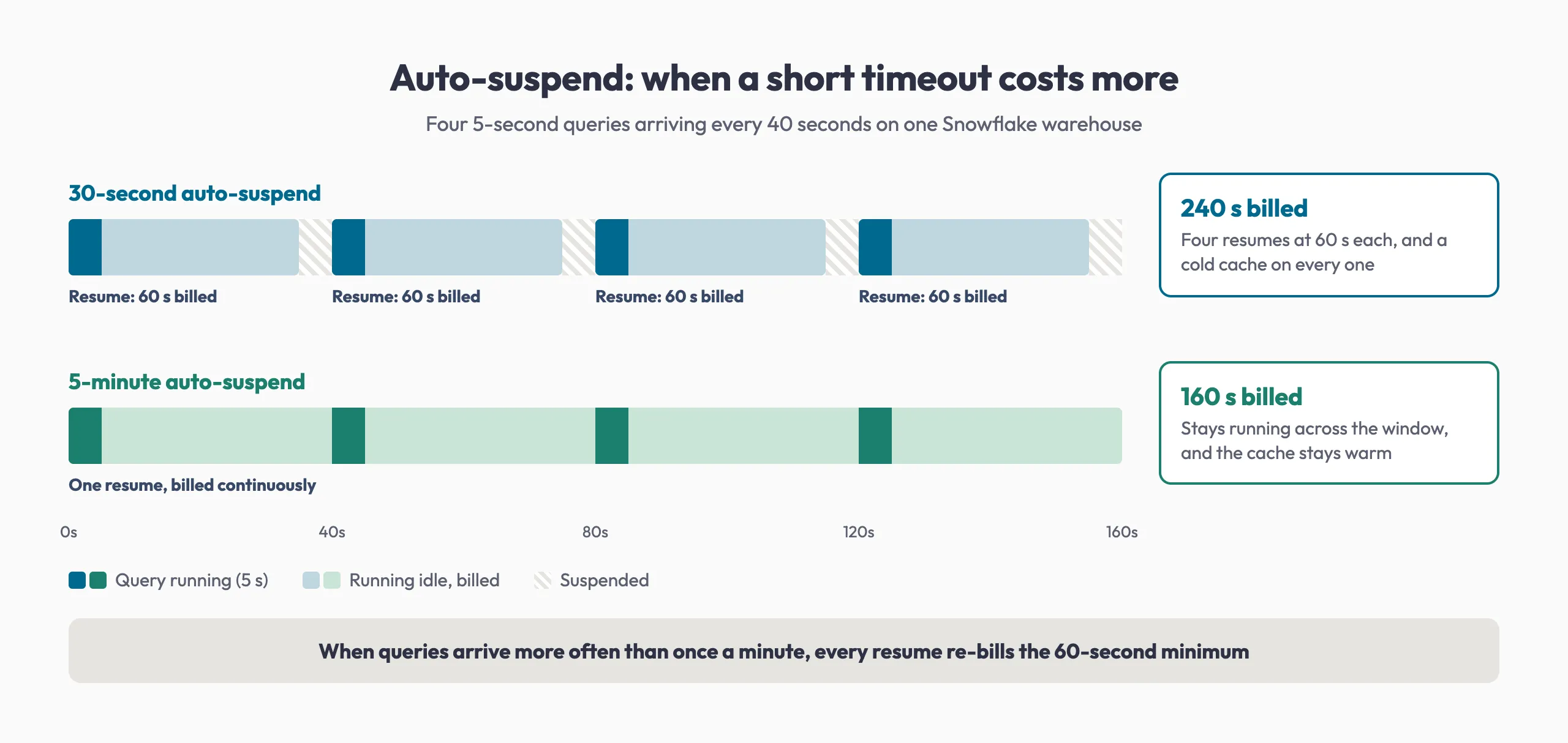
BigQuery capacity and bytes-billed limits
On-demand projects need a circuit breaker. Setting maximum bytes billed on the query job makes an over-limit query fail without incurring a charge. It is a job setting (console, bq flag, or API), not a SQL clause:
# BigQuery: fail any query that would bill more than 10 GB
bq query --use_legacy_sql=false --maximum_bytes_billed=10737418240 \
  'SELECT * FROM analytics.events WHERE DATE(created_at) = "2026-07-01"'
Capacity projects need the right baseline and ceiling. With BigQuery Editions, baseline slots are always allocated and always billed, so an oversized baseline wastes budget overnight. A max reservation size caps autoscaling spikes from unoptimized ad-hoc queries.
Matching compute configuration to workload
| Workload | Snowflake strategy | BigQuery strategy | Why |
|---|---|---|---|
| ETL and batch pipelines | 60-second auto-suspend | Dedicated reservation, low baseline, tight max | Batch jobs run in blocks; shut down right after |
| Ad-hoc and BI dashboards | 600-second auto-suspend | Autoscaling with a max cap, plus BI Engine | Users pause between actions; a warm cache keeps queries fast |
| Dev and testing | XS warehouse, 60 to 300-second auto-suspend | On-demand with a low maximum bytes billed | Limits waste from forgotten sessions |
These values track Snowflake’s own guidance. For more warehouse habits, see our 10 tips for getting more from Snowflake.
How to find your most expensive queries
You can’t optimize spend you can’t attribute, and both platforms expose per-query cost natively.
On Snowflake, the QUERY_ATTRIBUTION_HISTORY view reports the compute credits attributed to each query over the last year. (The credits_used_cloud_services column in QUERY_HISTORY covers cloud services only, not warehouse compute.) Grouping by query_parameterized_hash surfaces recurring patterns, where one fix pays off many times.
-- Snowflake: most expensive queries by compute credits (last 30 days)
SELECT
  qah.query_id,
  qah.warehouse_name,
  qah.query_tag,
  qah.credits_attributed_compute,
  LEFT(qh.query_text, 200) AS query_text
FROM snowflake.account_usage.query_attribution_history qah
JOIN snowflake.account_usage.query_history qh
  ON qah.query_id = qh.query_id
WHERE qah.start_time > DATEADD('day', -30, CURRENT_TIMESTAMP())
ORDER BY qah.credits_attributed_compute DESC
LIMIT 10;
On BigQuery, the INFORMATION_SCHEMA.JOBS view exposes bytes billed and slot time per job. Excluding SCRIPT statements avoids double-counting multi-statement jobs, whose parent row repeats its children’s totals.
-- BigQuery: most expensive queries (last 30 days)
SELECT
  job_id,
  user_email,
  total_bytes_billed / POW(1024, 4) AS tib_billed,
  total_slot_ms / 1000 / 3600 AS slot_hours
FROM `region-us`.INFORMATION_SCHEMA.JOBS_BY_PROJECT
WHERE creation_time > TIMESTAMP_SUB(CURRENT_TIMESTAMP(), INTERVAL 30 DAY)
  AND job_type = 'QUERY'
  AND statement_type != 'SCRIPT'
ORDER BY total_bytes_billed DESC
LIMIT 10;
Make query review a habit, not a one-time project. Snowflake’s Query Profile and BigQuery’s query plan show which step is expensive: a join exploding row counts, a SELECT * pulling unused columns, a subquery re-run per row. Add a cost check to your pull request template: did you read the plan, does the query prune partitions, is there a materialized alternative?
The part that’s easy to miss: multi-source cost leakage
Single-warehouse tuning doesn’t touch the costs that appear when teams query across platforms and cost centers. A question like “customer lifetime value by acquisition channel and product usage” often needs finance data in Snowflake and marketing data in BigQuery at once.
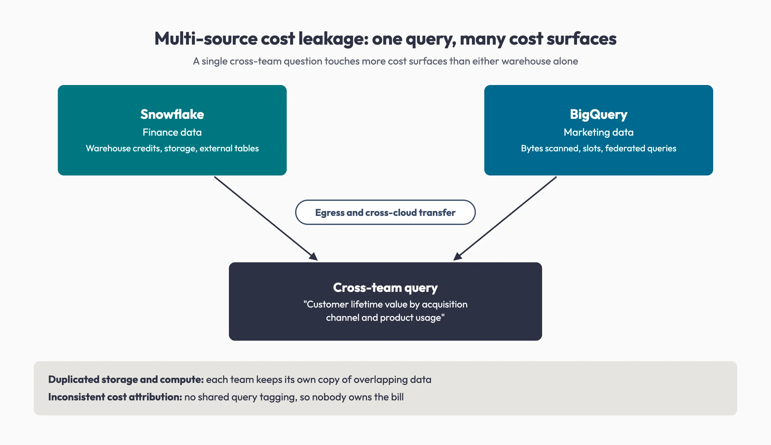
- Egress and cross-cloud transfer, billed separately and substantial when teams pull large tables across providers.
- Duplicated storage and compute, when each team keeps its own copy of overlapping data. (Within Snowflake, zero-copy cloning removes one common version.)
- Inconsistent attribution, when five teams share an untagged warehouse and nobody can say whose workload drives the bill.
- Federated query overhead: federated queries, external tables, and semantic layers reduce duplication but bring their own cost tradeoffs.
The practical fix: replicate aggregated summaries, not raw tables. If marketing needs a customer summary from the finance warehouse, materialize a 50 MB summary rather than federating against a 500 GB fact table on every query. This layer deserves its own effort once single-platform work is done, and the FinOps Foundation’s data cloud platform scenarios are a useful reference for it.
Where to start with Snowflake cost optimization
Make cost a design input, not an invoice surprise. Work in this order:
- Get visibility first. Set QUERY_TAG in Snowflake and job labels in BigQuery so cost is attributable to a team, pipeline, or project.
- Audit the top 10 most expensive queries from the last 30 days with the views above.
- Partition and cluster the tables behind those queries, not every table in the warehouse.
- Materialize any aggregation that runs more than once a day with the same logic.
- Right-size warehouses and reservations per workload using the table above, not one blanket setting.
- Set budgets and alerts per team: Snowflake resource monitors for warehouses, BigQuery budget alerts in Cloud Billing.
- Revisit multi-source flows for duplicated storage and compute.
When not to optimize
If a query costs less than $1 a day and runs reliably, leave it alone: two hours of engineering time at a conservative $100 an hour takes more than 200 days to pay back. Focus on pipelines costing more than $50 a day, patterns that repeat across pipelines, and costs that will hurt at two to three times today’s volume. FinOps is about ROI-positive decisions, not perfection.
Start this week: enable query tagging and pull your top 10 most expensive queries from the last 30 days. That single report will tell you more about where your budget goes than any best-practices list.
Frequently asked questions
What is the best auto-suspend setting for a Snowflake warehouse?
It depends on the workload. Snowflake recommends immediate suspension for task and batch warehouses, about five minutes for ad-hoc and data science work, and at least ten minutes for BI warehouses, where a warm cache keeps dashboards fast. The new-warehouse default is 600 seconds.
Does Snowflake charge a minimum when a warehouse resumes?
Yes. Snowflake bills warehouse compute per second, but each start or resume is billed for at least 60 seconds. When queries arrive more often than once a minute, a very short timeout re-bills that minimum on every resume and can cost more than keeping the warehouse running.
How do I find the most expensive queries in Snowflake?
Query the SNOWFLAKE.ACCOUNT_USAGE.QUERY_ATTRIBUTION_HISTORY view and sort by credits_attributed_compute. It attributes warehouse compute credits to individual queries for up to a year, though it excludes warehouse idle time and very short queries.
Do clustering keys always reduce Snowflake costs?
No. Clustering speeds up selective queries on large tables, but reclustering consumes credits. Snowflake recommends clustering keys mainly for multi-terabyte tables that are frequently filtered on the same columns.
Need help getting started with Snowflake cost optimization?
As a Snowflake Elite Services Partner, Atrium builds pipelines with cost as a design input: partitioning and clustering where queries actually filter, materialization where logic repeats, and warehouse settings matched to each workload. The teams that treat cost as part of engineering, not a quarterly cleanup, are the ones that keep scaling without surprises. Explore Atrium’s Snowflake data engineering services, or see how we deliver $1B in measured customer impact.