Cross-Industry Standard Process for Data Mining: Data Science for Business
CRISP-DM sounds delicious, but what is it? If you haven’t heard of CRISP-DM yet, you haven’t been following what machine learning and data science can do for your business. CRoss-Industry Standard Process for Data Mining (CRISP-DM) is a methodology businesses take in performing AI in an efficient, scalable way to meet stakeholder demand. Companies must act quickly in today’s environment, and that means their data and insights must move even quicker. CRISP-DM introduces six standard phases for data science in business:
- Business Understanding
- Data Understanding
- Data Preparation
- Modeling
- Evaluation
- Deployment
Over the next few minutes, I want to bring you up to speed on the power of this methodology with a mock business problem organized by the six phases above. That way, you can uncover how useful this will be in your own company’s context.
Business Understanding
Before we even see the data, we must understand the day-to-day problems a company and its people face. Our mock client is the Shailesh J. Mehta School of Management, Mumbai (SJMSOM). They are seeing incredible demand for their program thanks to the worldwide growth for careers in business. SJMSOM wants to be prepared as this growth continues. The school of management has a need for a robust lead scoring model in order to make the most out of their available resources when targeting students to take a specific Master of Business Administration level course.
A lead scoring model, in this case, will give predictive insight into the likelihood of a particular student taking the class. This model will take inputs, such as specialization, and provide a score from 0 to 100 on this likelihood. This will help provide insight for the school of management into where their resources will be best spent. There are several marketing efforts and contact campaigns in place, but there is currently no way to know how successful each method is.
Data Understanding / Data Preparation
Data understanding and preparation go hand in hand. First, you must view the data and get a feel for the underlying distributions, issues, labels, data types, etc. From this understanding, the data scientist can then fix any issues in the data preparation phase. But what is a data issue? Building robust models requires strict guidelines for incoming data. Aside from all of the assumptions about the data from a mathematics perspective, the model also does not perform well with missing data. In the real world, missingness is extremely common so there are several ways to handle this situation. Let’s see how I approach this in our mock example.
This dataset contains records about students, or leads, wishing to take a class at SJMSOM. There are 9,240 students in the collected data each with up to 49 variables pertaining to a range of details such as demographic and interest information. This course is a required course for Masters in Business Administration (MBA) students as many students (5,204) come from management or business-focused backgrounds. The goal of this dataset is to determine a lead propensity score using the variable, Is Won?. A lead for the school of management can be defined as a student who has applied for the course. The school’s sales team then targets this student and helps them through the sales process with lead stages. The student ultimately either takes the course or decides not to at some point in the sales process; therefore, the student is either “won” or “lost”, hence, “Is Won?” This data will be used to create a model for new lead propensity scoring.
Missingness of data is a major problem in this data. Only 21 variables have less than 20% of missing values. Even worse, 18 variables have more than 60% of data missing. I engineered a profile strength variable to retain some information from 16 of the variables, while I dropped other columns completely. The new profile strength variable is a way of scoring a student’s application on completeness. If a student did not care to take the time to properly complete the application for the class, my hypothesis is the lead will convert less frequently than a more complete application. For a single record, a complete application would receive a 16 (one point for each completed part of the application) while an application with nothing filled out would receive a score of zero. Table 1 shows an example of a calculation for profile strength.
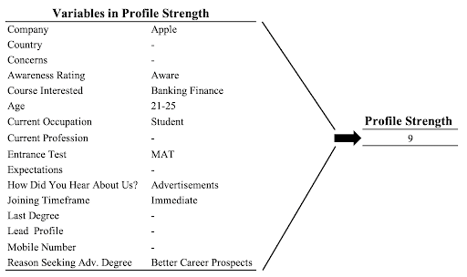
Table 1. Example of Profile Strength calculation.
This is a great time to introduce a topic called exploratory data analysis, or EDA. EDA gives a visual representation of the data. This process is the most efficient way to quickly see potentially useful relationships at play within the dataset. For the sake of brevity, I will only display one example of EDA, but the full analysis considers all potential relationships. Of course, modeling the data is the best way to create inference from the data, but EDA provides a starting point for further analysis in model building. Figure 1 shows how much the profile strength distribution changes based on a lead being won or lost. This shows visual evidence of a relationship between Is Won? and Profile Strength. If there had been no relationship at all, the two boxplots would look like mirror images of each other.
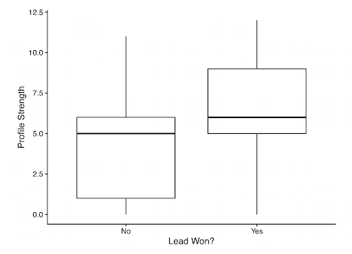
Figure 1. Boxplot of Profile Strength.
Along with EDA, I used several other techniques in data understanding and preparation such as variable transformation and distribution analysis. Once this is complete, the dataset is left with the 13 variables in Table 2. Is Won? is the variable I wish to predict.
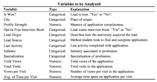
Table 2. Variable Description.
Modeling
It took a lot of work to get to this point, but we are finally able to create plausible methods for modeling this data. The lead scoring model can now start to be identified for SJMSOM. The outcome variable in this case is Is Won? which is a binary, categorical variable (Won or Lost). This data is most appropriate to be fit with one of two models.
The first model is a logistic regression approach to produce lead propensity based on the features I have identified. This model was rigorously tested to ensure the model gives accurate predictions on future student leads. A final model will be able to produce lead propensity in terms of a probability of winning the lead. On top of the predictive insight, the model will allow SJMSOM to know how each variable and factor impacts propensity.
A second model will invoke a decision tree based method called a random forest. This technique is at the forefront of predictive modeling, but one downside is the loss of the same level of interpretability that the logistic model provides. This model will produce a propensity score as well as a prediction of “Win”/“Loss”, but the impact of each variable and their factors is not as in-depth as the logistic model is able to provide.
In case you are new to the idea of a random forest, imagine a bunch of decision trees. Figure 6 gives an example of a decision tree. A random forest scales this idea up. Instead of producing one tree, hundreds of trees are developed in a similar manner. With the optimal random forest created, I can move to evaluation between the two models created.
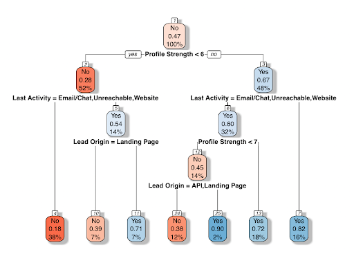
Figure 2. Example of a decision tree using this data. Each bubble gives three values: a word, a number, and a percentage. The word is the predicted outcome at that specific point, or node, in the tree. The number is the propensity score at that node. The percent is the amount of data in the training set that made it to that specific node. Below each bubble is a decision. If the logical expression is true, the record continues to the left in the tree. Once a record reaches a final point with no additional decisions, a final prediction is given.
Evaluation
Evaluation is a key aspect of finding the appropriate model for your specific business needs. It is important to build both of these models and test their predictive ability against each other. This will be done by splitting the data into a training set with 70% of the original data and a testing set with 30% of the data. This will allow SJMSOM to be confident in the output from these models.
Each model has been developed using training data. The university gave me ample data to be able to provide a look at predictive power on a test data set. The logistic model was able to predict on the training data with accuracy of 74.92% while the random forest was able to predict the training data with 87.37% accuracy. With the test data, the logistic model was able to predict accurately 75.05% of the time while the random forest model was able to predict correctly 77.35% of the time. This is very close. If predictive accuracy was the only concern, the random forest would be desired, but the university also needs to know specific contributors in order to drive higher lead conversion. For this reason, the logistic model will be best for SJMSOM as it provides a good balance between predictive accuracy and inference capability. The full report gives a deeper look at the inference capability, but in summary, industry, profile strength, activity, origin, and free book decision are key indicators of success.
Deployment (Salesforce Implementation)
With a model decided on, it is time to deploy this model. A model by itself is useful and provides insight, but a model that provides real time insight for each individual salesperson on your team can turn out to be invaluable. This is exactly the capability Salesforce Einstein Discovery delivers.
I was able to provide insights to SJMSOM salespeople through sorted listviews (Figure 3) and side card views of potential drivers (Figure 4). The list view will provide a list of all student leads and sort by lead score. This will allow a salesperson to either avoid low scoring leads and focus on converting higher scoring leads, or dig into why a lead is scoring so low with the hopes of a discovery of a systematic change that could help the entire sales team. If a salesperson wants to dive into a specific record, they have the ability to drill in and gain feedback and recommendations on what is working as well as what is not for that particular student. I was able to build and deploy all of this through the power of Salesforce Einstein Discovery.
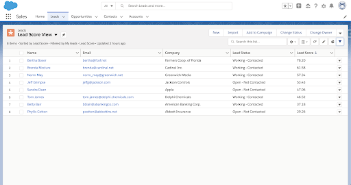
Figure 3. Example listview sorted by lead score.
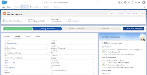
Figure 4. Example record specific recommendations.
Conclusion
Through this example, we were able to see a mock analysis of how CRISP-DM can be used to solve a real business problem. This methodology provides a consistent framework to solve a wide range of problems. The purpose of this methodology is to allow more time to be spent on analyzing a problem rather than reinventing the wheel every time we want to apply artificial intelligence to our business decisions.
We saw first hand the impact of model building as well as the power of deploying a model to our end users within the business. This will be used to provide insights to the sales team in an intuitive, efficient way. I hope you can take these ideas and relate them to your own business needs. The data science team at Atrium can help make these solutions a reality for your company. And to see a more in-depth view of this example, check out our whitepaper here.
References
RockBottom. (2016, August 19). Leads dataset. Retrieved March 01, 2021, from https://www.kaggle.com/ rockbottom73/leads-dataset.