Exploring Data Classification: NN, K-NN, Linear, SVM, Softmax, and Neural Networks
Nowadays, the use of data in the field of technology is growing exponentially. Lots of companies are working day and night on them. But the question is why do we need data classification?
First we have to understand what data classification is. Data classification is a process of predicting the class (labels/categories) of the given data points. And we classify the data so that we can understand and estimate the behavior of the data in a better way. There are lots of classification algorithms which are in use. But we can’t say that one classification algorithm is better than the other. It all depends on the application and nature of the problem you are dealing with. Each algorithm uses a classification predictive model which takes some input variables and produces the discrete output.
There are numerous scenarios where we can use classification algorithms. Some of the use cases are customer segmentation, customer acquisition, customer retention, salary classification, etc.
Let’s take a dive deep and understand the different types of classification algorithms.
Nearest Neighbor
It is a non-parametric classifier as the entire training set are the model parameters. Let us take a pictorial view to understand the concept clearly. In the diagram attached below we can see two types of objects, one having the shape of a star and the other one is triangular. There is one object which is square in shape and is denoted by “New example to classify.” This algorithm finds the distance between each and every training example with the “New example to classify” and returns the label of the nearest one. So, the label of the test example is defined as the label of the training example nearest to the test example.
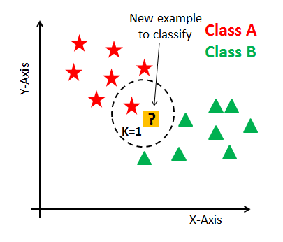
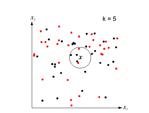
K Nearest Neighbor is the extended version of Nearest Neighbor. It needs the k-nearest training data label to decide its test data label. We can use this model while we are working on economic forecasting, data compressions, customer acquisition, customer retention, and genetics. This is done by observing the behavior of a particular object and finding which object has the closest similar behavior and what its label is.
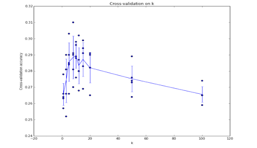
In cases when the training dataset is small, people use complex techniques for hyperparameter tuning called cross validation. In this technique we split the train data into train set and validation set and further use validation set for hyperparameter tuning. In general, you can say the validation set works as a test set while training the train set data. This is because we know the label of validation set data and also predicting it on the basis of features, so that we can compare the actual and predicted value.
The value of K can be determined by visualizing the graph of cross validation accuracy
- K.
Linear Class
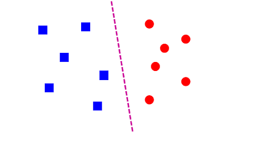
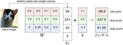
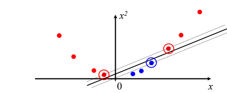
It is a parametric classifier which depends on two parameters (W,b). The line which we are seeing in the picture is called the hypothesis line, which depends on parameters called weights and bias. It uses linear function to separate the class. The linear function looks like: F(xi,W,b) = Wxi+b
It uses squared error cost function, which is the summation of the mean of the square difference between the actual and predicted output variable. Our final goal is to minimize the cost function by changing the parameters to get the best hypothesis.
Let us take an example of an image classification. Suppose we have to classify three classes.
- Xi is all of its pixel values flattened out in single column (let’s suppose you have an image whose length is 32px and width is 32 px and it consists of three-layer RGB so the total dimension of Xi is 1×32*32*3).
- W is one of the parameters called weight matrix with a dimension of Kx32*32*3. Here K is the number of classes. In our case it is 3.
- And b is the second parameter, known as bias term with a dimension of kx1
The function returns the score value of each class. The test data belongs to the class which scores the most.
Support Vector Machine
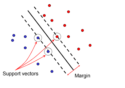
A classification technique which is used very generally. It is very much similar to a linear classifier and is based on maximum marginal principle. When the data is linearly separable there may be more than one hyperplane.
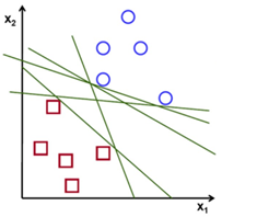
To find the best separator, one has to find that hyperplane which maximizes the margin between positive and negative examples. It means we have to find that hyperplane which bisects the distance between positive and negative class so that both classes have a maximum distance with the hyperplane.
It is used in various image classification problems like gender detection, biometrics. It is widely used for identification of biological sequences.
Non-Linear SVM
The original input space mapped to some higher dimensional feature space where the training set is separable.
Let’s take an example with some dataset points in 1D for a better understanding.
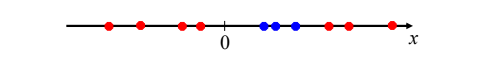
Here we can’t separate this dataset with a single linear separator, but as we increase the dimension we can see that it can be easily done.
Softmax Classifier
It is one of the popular classifiers similar to SVM classifier. Softmax classifier is the generalization to multiple classes of binary logistic regression classifiers. It works best when we are dealing with mutually exclusive output. Let us take an example of predicting whether a patient will visit the hospital in future. We can’t predict it mutually exclusively as one patient can visit the hospital because of various issues (e.g., heart issue, neuron issues, etc.) but while predicting the character of handwritten digits or working on irises datasets we are dealing with mutually exclusive output — and softmax classifier works best in these cases.
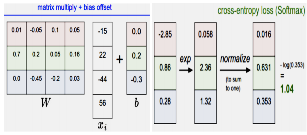
Loss function measures how compatible the given set of parameters with respect to ground truth value. Unlike SVM classifiers which use hinge loss, it works on cross entropy loss.
We can view and analyze the loss function by looking at the image below. It uses the output of hypothesis and passes it through exponential function and does normalization and further passes it through logarithmic function to analyze and minimize the loss.
Unlike SVM classifier, which treats the output as the score of each class, softmax classifier gives something additional. It gives you the normalized class probabilities. So it is easy for humans to visualize.
Neural Network
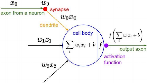
The area of neural networks comes into picture from how humans can recognize the object. The basic computational unit of the brain is neurons. Each neuron receives an input signal from dendrites. It provides output signals along the axon. The axon branches out and connects via synapses to dendrites of other neurons.
The main function of the activation function is to add non-linearity in the network.
Let’s discuss the perceptron update rules to get the picture clearer.
- Initialize the weight randomly.
- Cycle through training examples with multiple iterations (epoch).
- For each training instance with level y classify with current weights.
- If the classified label is correct it’s good, or else do the modification in weights.
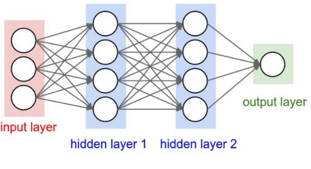
Number of neurons (excluding input layer) is 4+4+1 = 9.
Number of learning parameters is ([3*4+4*4+4*1] = 32 weights , [4+4+1]=9 bias) = 41.
Some Important points related to neural networks for understanding the network:
- The input layer contains the features of the data (features are the properties which define the data).
- Initially the random value of weights is assigned with some bias values.
- Then the feed forward neural network runs and checks the output label of the classifier.
- To minimize the error between true and estimated outputs we do some changes in weights.
- The weight is updated with the help of gradient descent.
- Then it runs the back propagation, which means gradients are run from output to input layer and combined using chain rules.
- We update the weights and bias value of the network. And after some epoch (i.e., iteration) we minimize the loss.
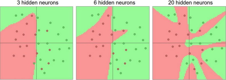
With the increase of hidden layers we can make extremely powerful models in neural networks. We can visualize the same from the image below. It is used in various image and speech recognition tasks. With the help of Cnn and Rnn we can perform a lot in the field of deep learning.
Classifier Pros and Cons
NN/KNN
- Fast at training
- Performs well with large datasets
- Can distinguish two or more than two objects
- Memory inefficient
- Slow at test time
- Optimum
- Value of k is not known, which results in a bad model (less accurate)
Linear
- Fast at test time
- Depends on fewer parameters (weights and bias only)
- Slow in training time
- Data may not be linearly separable
SVM
- Kernel based framework is flexible
- Global optimal solution
- Works well with less data
- Memory inefficient
- Computationally slow
- Multiclass SVM can’t be used directly
Softmax
- Good prediction on training data
- Small loss
- Gives probability, easy for humans to interpret
- Optimal loss is a challenge
- Multiclass classification is mutually exclusive
Neural Network
- Build extremely powerful model by hidden layer
- General function approximation framework
- Flexible
- High computational power required
- Memory inefficient
- Hard to decode theoretically because of complex network
Considering Data Classification Techniques
After going through these classification techniques you get the basic idea and abstract view of it. It is very important to understand each type of classification model so that you can select the best prediction model for a particular use case.
Classification techniques are also very popular in the visual world. Lots of big companies and startups are working a lot with visual data as well. You might have seen some graphical user interface where by giving the input as image it describes the image in a sentence as an output. It is not magic — they use image-based segmentation on the image to classify each object on the image and further use some deep learning concept (RNN) to relate each object and frame a sentence.
Subscribe to our blog for more technical information and industry news